Optimization of a plant cooling system design

To optimize a plant cooling system, let’s first look at using system simulation software to obtain accurate sizing of a feed water pump. Simulation software can reduce system oversizing and increase safety and efficiency. For analyzing a plant cooling system design, simulation software that is able to model thermal and fluid dynamics is needed.

Then, simulation analyses will be used to integrate the chilled water side of the cooling system into the design, consider various heat-exchanger options and determine cooling system expected power and energy use, creating a baseline model and better understanding of lifecycle costs.

Finally, using the baseline design, optimization software will be used to further refine the design to the most optimal arrangement for the plant cooling system.

Get started

Pumping systems ensure fluids reach their destination through often-complex flow distribution networks. However, for most industry sectors, pumping systems usually have the highest power consumption of any process system. Estimates run that operation and maintenance often make up more than 80% of lifetime pumping system costs.

Initial pump sizing usually comes early in the design process. All data and final routing may not be available, but it’s possible to estimate based on initial layouts (see Figure 1). The model is composed of several heat sources: a diesel generator, ancillary equipment, scavenger oil cooler, lubrication oil cooler and engine jacket. A feed water pump also is part of this cooling loop. The entire loop interacts with a cooling loop that pumps seawater through a heat exchanger.

System constraints include the following:

• Limit of 80 °C on temperature, anywhere in the system.
• The seawater system was finalized so no changes could be made to the pumps or piping on that side, only to the heat exchanger through which it interacts.
• Due to the layout and constraints, maximum pipe size was a 200-mm, schedule-40, nominal pipe size.

With these constraints, what parameters could be changed?

First was pipe size. To keep things simple, consider a schedule 40 stainless steel between 100- and 200-mm piping at 25 mm nominal increments, with 7-inch or 175-mm excluded due to lack of ready availability.

Second, an initial estimate gave an expected flow rate of 0.0631 m3/s, which is about 1,000 gal/min. However, to ensure proper pump operation under different flow rates, a sweep from 0.0158 to 0.0788 m3/s, or about 250 to 1,250 gal/min should be considered.

Finally, the heat exchanger was looked at. It’s a shell and-tube configuration with either two or four passes. Its length will be from 1 to 5 m.

Asking a few questions can lead to the best solution. What is the overall system pressure drop? Which pump options fit the system? Finally, what is the power requirement of the selected pump?

Calculating system pressure drop

In this analysis, we focus on the cooling system’s closed-loop portion, excluding the seawater side. To determine losses in the system over a range of flow rates, the pump initially can be configured as a flow source and pressure sink. This allows forcing a flow rate on the system so that simulation software can calculate required upstream pressure based on the outlet pressure and system component accumulative losses.

Certain fixed data is assumed constant from design to design. For the pipes, a roughness of 0.025 mm can be used. Piping lengths vary from five to 35 meters. For utilities, a loss coefficient of 0.2 can be used. Other data varies, including pipe diameter, volumetric flow rate, orifice diameter and flow area of the utilities.

To accurately estimate system performance, let’s look at four different pipe inner diameters, corresponding to 100, 125, 150, and 200 mm schedule-40 pipe. Also considered were five different flow rates from 0.0158 to 0.0788 m3/s (see Figure 2).

Running virtual experiments

Here is where major software benefits apply. Running many scenarios is simple and fast. We create variable parameters and assign them to components in place of specific numbers. We can then configure the design of experiments to vary these values from run to run.

Once the variables are configured, the software sets up the experiment. We determine how the variable parameter data is to change. For pipe diameter, discrete values are used, which allow entering specific numbers. This is helpful when there isn’t a distinct mathematical pattern to the entries such as for pipe schedules. For flow rate, we set a start- and end-value and select the number of values; in this case, five.

The software then determines the values and creates the run matrix of a full factorial, in this case, 20 total, which runs in just under 15 seconds.

From the experiments, results are exported directly to a spreadsheet for graphing of the four possible system curves. The 100-mm option resulted in far too high resistance, ruling that option out immediately. As for the 125-, 150-, and 200-mm options, the system curves look reasonable, so a decision will likely be based on weight and operating expense.

From initial heat load calculations, we know the system should be run at around 0.63 m3/s. If a vertical line is drawn on the graph, we can see where that intersects with our system curve (Figure 3). Drawing a line horizontal to the y-axis determines what the required head rise from the pump will be. As an example, for the 125-mm option, it would be about 22.1 meters. This information helps narrow down the pump options to those that have a rated head and rated flow as close to these values as possible.

Figure 4: Pump and system curves. Courtesy: Mentor[/caption]

Although pump 101A didn’t intersect exactly at the desired flow rate, it was close and slightly to the right, so it could provide enough rate and some buffer.

Selecting 101A, we can input the pump data for the manufacturer can be inputted and an analysis run to see how it operates in the model. The results shows the intersection point or operating point is at a slightly higher flow rate than the flow rate of 0.063 m3/s; but not by much, which meant the head rise is going to be slightly lower than the rate value. But again, not by much. This means that the efficiency is going to be slightly lower at 74.9% versus the stated 77%. Ultimately, the required power would be just over 8 kW.

The first step to optimize the design of a new industrial cooling system for both cost and performance has been demonstrated. A traditional design process to build the thermo-fluid simulation model is perfectly valid for meeting engineering constraints. However, these solutions could still be cost-inefficient. Further analyses will refine our options.

Heat exchanger options

Let’s now look at how simulation analyses can be used to consider heat-exchanger options and determine expected power and energy use of the plant cooling system, working to model and optimize lifecycle costs.

With the pump sized and the seawater circuit incorporated into the model (Figure B1), let’s look at heat exchanger data. The simulation software uses empirical data to define the heat exchanger. This includes thermal duty, used in the utilities, hot or cold stream temperature difference, or effectiveness or nascent number, specified as single values or as varying with flow rates. These are usually good options, if you have the test or manufacturer’s data.

However, if that’s not an option, or for greater control defining the heat exchanger, the geometry can be specified. In this case, selection of heat exchangers can be based on the VDI heat atlas used in the power generation and process industries, as well as an advanced option, which caters more toward designing automotive heat exchangers. In this example, the geometry-based option from the VDI heat atlas is used.

The first decision is the type of heat exchanger. To look at the difference between a two-pass and a four-pass, shell-and-tube, counter-flow heat exchanger, the tube inner diameter and thickness can be fixed and the tube length, number of tubes and shell diameter, which is a function of the number of tubes, can be varied. Five different tube lengths and five different values for the number of tubes can then be compared.

This provides 25 experiments, which, as with sizing the pump, solves in about 30 seconds using the virtual experiments. This provides 25 runs for each heat exchanger option, or 50 total.

Once complete, results are exported to Excel to graph as shown in Figure 5. Not surprisingly, as tube length for a given number of tubes increases, the calculated outlet temperature decreases, which is also the case if the number of tubes increases while length stays the same. Increasing tube length has a much greater effect on outlet temperature than increasing the number of tubes. For example, this time, we’ll start with 50 one-meter length tubes and increase the number of tubes to 100, then go from an outlet temperature of 105 to 82.5 °C.

Figure 6: Temperatures were lower than for the two-pass design. Courtesy: Mentor[/caption]

Power and energy use

With pump and heat exchanger size in hand, we can optimize the system based on cost, while still meeting the original requirements. For the model’s cost portion, an Excel spreadsheet linked to heat is used. The main impacts bearing on cooling system lifecycle costs are initial purchase cost; piping, pump and heat exchanger costs; maintenance costs for each over 25 years; and energy cost to run the plant as expected. Not included are projected downtime, environmental costs and decommissioning, though they could be included.

Using these numbers, a baseline using the original model (Figure 7) is established. Cost is just over $382,000, along with other important notes in terms of temperature pressures and power. As mentioned, most of these costs are for electricity and maintenance. How might these costs be reduced?

With a parametric study approach, combining the four input variables represented 980 unique simulations, and that’s with no direct connection to costing functions. Significant manual post-processing would determine the best option but there must be a better option.

Streamlining the process

Next, a design optimization tool can improve the initial simulation model and design analysis based on design goals and costing functions, resulting in a smaller study size, which saves time and optimizes the design.

To do so requires streamlining the virtual product-development process. Today, most companies begin building their virtual prototype simulations by connecting their CAD, CAE, and perhaps costing tools. Then they recreate product operational tests for the virtual prototypes. Once confident with the virtual prototype performance predictions, the design is improved by making modifications manually or with a design of experiments approach, as seen above. Finally, the resulting design may be assessed for robustness before releasing the product for production.

Many manufacturers allocate most of their modeling and simulation resources to building and testing virtual prototypes. However, the greatest value from these tools comes from understanding and improving designs. How can this be improved?

Validated or robust CAD and CAE models can be rebuilt easily with changes in design variables. Simulating one full design prototype using a variety of CAD or CAE tools can be automated, even with a costing model included. This can be as simple or complicated as needed to fully simulate the behavior of one design or one virtual prototype.

Once the process is automated, after each task is defined the process is simulated in a high-performance computing environment so that many variations can be quickly explored. Some tasks may be assigned to Windows computers, others to Linux clusters and still others to external cloud resources.

Modern direct search techniques can efficiently explore the full nonlinear design space and quickly discover better designs, with no need for surrogate models.

Last, we examine the sensitivity, robustness and variable interactions of the best designs to gain insights and understand how performance will be affected by normal manufacturing tolerances. This is the state of the art and modern design exploration today.

Even if software solutions offer hybrid strategies, they still contain predefined algorithms rather than adjusting to the problem at hand. What’s needed is a tool that knows all the strategies, holds all the parts, and can be tailored according to the design approach and criteria. The design exploration software framework  used for this analysis is both hybrid and adaptive and eliminates the previously described issues with the traditional approach.

For this case, the simulation model specified was created in the Excel spreadsheet along with the baseline conditions. The software then efficiently searched the design space to find an optimal solution with fewer simulations. Let’s look at some improved designs.

For the initial design, three different things were optimized (Table 1). The pipe diameter went from 125 to 150 mm. The pump size was cut in half, and the heat exchanger size changed from three meters to one meter. The maximum temperature and pressure were still where needed, and pump power decreased significantly. This was caused by a decrease in the pressure rise required and in the flow rates, allowing a smaller pump to be used. Pump size reduction also reduced electricity use as well as required maintenance.

The software indicated the piping install and purchase price would increase. However, even if upfront costs increase, in the long run, nearly $180,000 is saved. This a good optimization when considering the life of the design.

Using even more variables

However, was it safe to assume all the pipes must be the same size? Could some of the smaller paths that require less duty, and thus should require a lesser flow rate, be a different size? How would that affect the cost and selection of pumps?

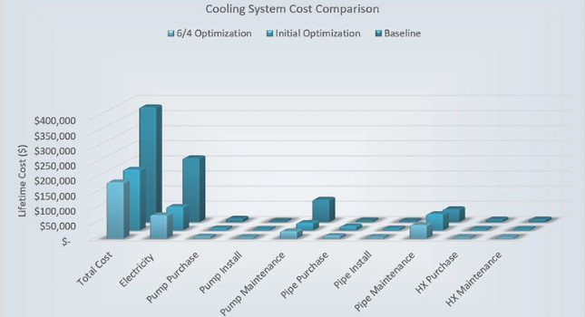
What if, instead of having six inches or 150 mms throughout the system, 150 and 100 mm or six and four inches were used, leaving the pump and heat exchanger the same size? The pump power could be maintained. The maximum temperature was still about the same. Pressure increased a bit, but negligibly. However, the savings was about $17,000, mainly because of the decrease in the pipe purchase and install (Figure 8).

The software can also weight options for buying two pumps to run in parallel. That means twice the purchase cost, but it could be assumed that the install and maintenance would be only 1.5 times. With this option, we’ll split them in half because our concern is making sure flow rate stays the same and pressure is about the same, which is what we can do with a parallel configuration.

Now instead of using a pump that requires almost 3 kW, we can use pumps that use less than 1 kW. The maximum temperature is a little bit higher, but the pressure is a little bit lower. This means that, although these pumps are split, the performance isn’t the same. This is justifiable if it’s in the same engineering acceptable range, because the savings would be about $30,000. Most of that savings comes from the electricity over the system’s life, as well as a little on pump maintenance.

Final words

This article demonstrates how to optimize a new industrial cooling system design for cost and performance. A traditional design process was used to build the thermo-fluid simulation model, necessary to meet engineering constraints. Although these solutions may be good, they could be more costly than they need to be. By combining the model with a design optimization tool to manipulate the model in conjunction with a cost calculation, optimal arrangements were discovered, and system design further refined. In this example, more than $225,000 was saved. Moreover, the time to perform this versus doing it in a parametric study is much less.

Today’s modern design tools can be combined in new and interesting ways to produce better, more efficient products for today… and tomorrow.

The system simulation software used was Siemens Simcenter Flomaster.

Siemens HEEDS design exploration software was used to further refine the design.

Do you have experience and expertise with the topics mentioned in this content? You should consider contributing to our CFE Media editorial team and getting the recognition you and your company deserve. Click here to start this process.